


A server room that runs too hot will not stay reliable for long. Excess heat degrades components, triggers abrupt shutdowns, and shortens the working life of expensive hardware. At the heart of every effective thermal management strategy sits a single critical figure: cooling capacity. Getting that number right determines whether a precision air conditioning system will quietly protect operations or become a costly mismatch. Understanding how to calculate this capacity—and what makes it fluctuate—is an essential skill for anyone responsible for mission-critical environments.
What Cooling Capacity Actually Means
Cooling capacity measures how much heat an air conditioning unit can extract and reject from a space within a specific time period. The standard international unit is the kilowatt (kW), though some specifications still reference kilocalories per hour (kcal/h). One kilowatt equals approximately 860 kcal/h. This number directly defines the unit’s ability to offset thermal energy and hold supply air at the target temperature. If the calculated capacity falls short of the real heat load, hot spots will form. If the capacity is grossly inflated, the system will short-cycle, causing humidity instability and unnecessary electrical consumption. Precision matters because the goal is not just cooling—it is stable, continuous cooling matched exactly to demand.
Factors That Shape Cooling Requirements
Several variables combine to produce the total heat load inside a data center. Ignoring any one of them will distort the final capacity figure.


Room Area and Physical Envelope
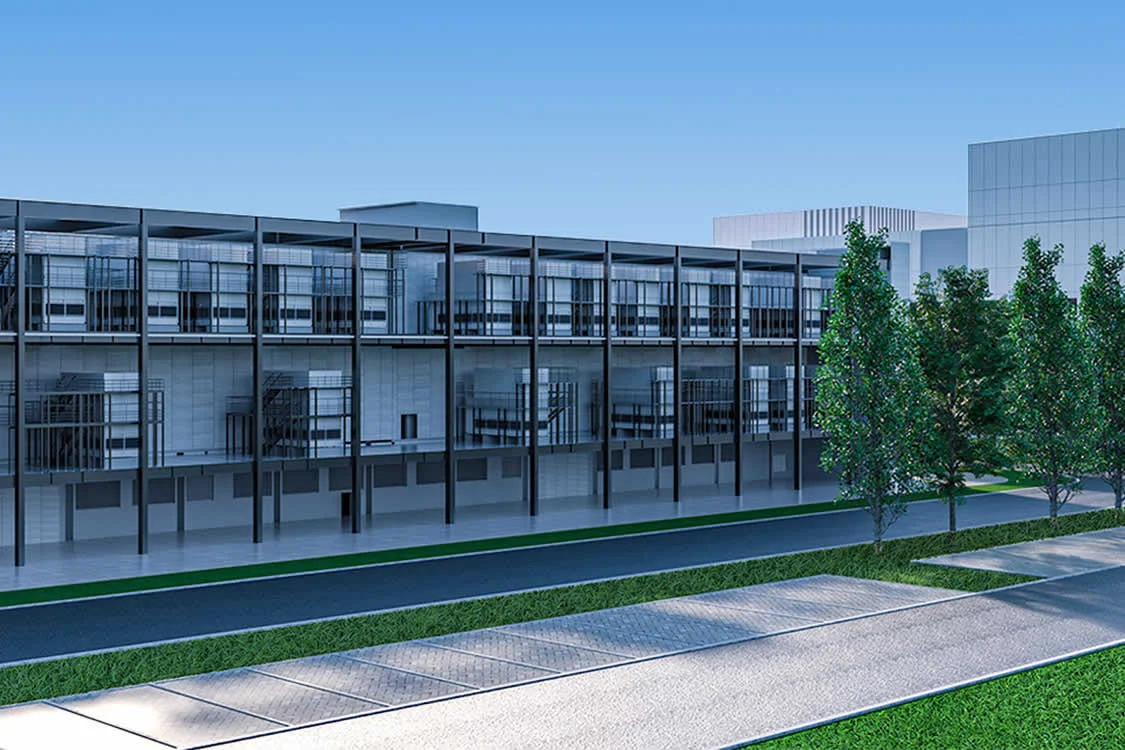
Floor area provides a baseline metric. A widely used reference point suggests allocating 0.1 to 0.15 kW of cooling per square meter. This factor covers the conductive heat gain through walls, ceilings, and floors. Ceiling height, insulation quality, and exposure to exterior sunlight or adjacent hot zones all modify this base load. A room with large windows facing the afternoon sun, for instance, will soak up far more energy than an interior, windowless space. The area-based estimate serves as a starting point, but it must be adjusted for the specific architectural context.


Heat Dissipated by IT Equipment
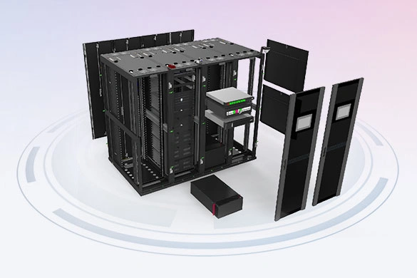
This is typically the dominant and most dynamic component. Servers, storage systems, networking switches, and uninterruptible power supplies convert virtually all of their electrical input power into heat. A rack drawing 5 kW of electricity effectively injects 5 kW of thermal energy into the room. Nameplate ratings on equipment often overstate real draw, so actual measured power consumption—captured at the rack power distribution unit—yields a much more accurate heat dissipation figure. Summing the continuous electrical load of every piece of active hardware transforms an abstract equipment list into a concrete thermal figure.

Ambient Temperature Conditions
The temperature of the surrounding environment works on two fronts. It drives the conductive heat transfer across the building envelope: the hotter the outside air, the more heat leaks into the conditioned space. At the same time, higher outdoor temperatures raise the condensing pressure in the refrigeration circuit, reducing the effective cooling output of the unit itself. Seasonal extremes matter. A system sized for mild weather might falter when an external heatwave pushes both infiltration and condensing temperatures upward. The design ambient temperature must reflect the worst-case scenario the site will face.

Airflow Distribution and Circulation Quality
Cooling capacity on paper means nothing if cold air cannot reach equipment intakes. Poor airflow patterns—obstructed raised-floor pathways, misplaced perforated tiles, uncontained hot exhaust recirculating into cold aisles—create hot spots even when the room’s total cooling output appears adequate. Inefficient air circulation forces the cooling system to work harder, driving down its effective capacity. Sealing gaps, arranging racks into hot and cold aisles, and managing airflow with blanking panels all improve the utilization of every kilowatt of installed cooling. Without proper circulation, part of the capacity is wasted on mixing losses rather than meaningful heat removal.
Methods for Calculating Cooling Capacity
Three distinct approaches dominate the industry, each suited to a different stage of planning and operation.
Empirical Estimation
This quick-sizing method applies simple rules of thumb, often based on area, estimated equipment count, and environmental factors pulled from lookup tables. An operator might multiply total square meters by a per-meter load factor, then add a flat allowance for each rack. The appeal lies in speed: rough figures appear almost immediately. The weakness is imprecision. The method layers generic safety margins on top of assumptions, frequently overestimating true demand by a significant margin. Empirical estimation works well for initial budgetary planning but should not be used to finalize equipment specifications.

Detailed Heat Load Calculation
For accuracy, the total thermal burden is broken into its constituent parts and summed. The process accounts for conductive gains through walls and glass, the full electrical draw of IT and ancillary hardware, heat from lighting and occupants, and solar radiation where applicable. Each heat source is converted into a kW value. The sum yields the peak cooling load—a defensible, site-specific number. Although this method demands careful data collection and arithmetic, it produces the reliable foundation needed for equipment selection, avoiding both dangerous undersizing and wasteful oversizing.
Dynamic Balancing
Modern precision cooling systems can go beyond static calculations by adopting adaptive, sensor-driven operation. Temperature probes distributed across cold aisles and return air paths feed real-time data to the unit’s controller. Variable-speed compressors, electronically commutated fans, and modulating expansion valves adjust output moment by moment to follow the actual thermal load. This method does not replace the need for a properly sized base system, but it transforms how that capacity is delivered. Dynamic balancing cuts energy consumption during off-peak periods, prevents temperature swings, and compensates for gradual load changes without manual intervention. It demands sophisticated controls but delivers the closest alignment between cooling supplied and heat generated.
Selecting an air conditioning system without a clear calculation of required cooling capacity is a gamble that no data center can afford. The process begins with defining what capacity means, moves through a careful review of area loads, equipment heat, outdoor conditions, and airflow efficiency, and concludes with a methodical calculation matched to the stage of the project. Whether using empirical estimates for early discussions, detailed thermal math for final design, or dynamic controls for ongoing optimization, the objective stays the same: precisely enough cooling to keep critical systems stable, energy consumption in check, and operating costs under control.